Computational graphs and gradient flows
Prerequisites
To best understand this article, you should know about:
- Calculus:
Partial derivatives.
What is a computational graph?
As colah said quite nicely: computational graphs are a nice way to think about mathematical expressions.
For example, consider the expression \(e = (a+b) ∗ (b+1)\).
There are three operations here: two additions and one multiplication.
- To help us talk about this, let’s introduce two intermediary variables \(c\) and \(d\), so that every function’s output is a variable. Thus:
\(c = f_1(a, b) = (a + b)\)
\(d = f_2(b) = (b + 1)\)
\(e = f_3(c, d) = (c * d)\)
To create a computational graph, we make each of these operations, along with the input variables, into nodes. When one node’s value is the input to another node, an arrow goes from one to another.
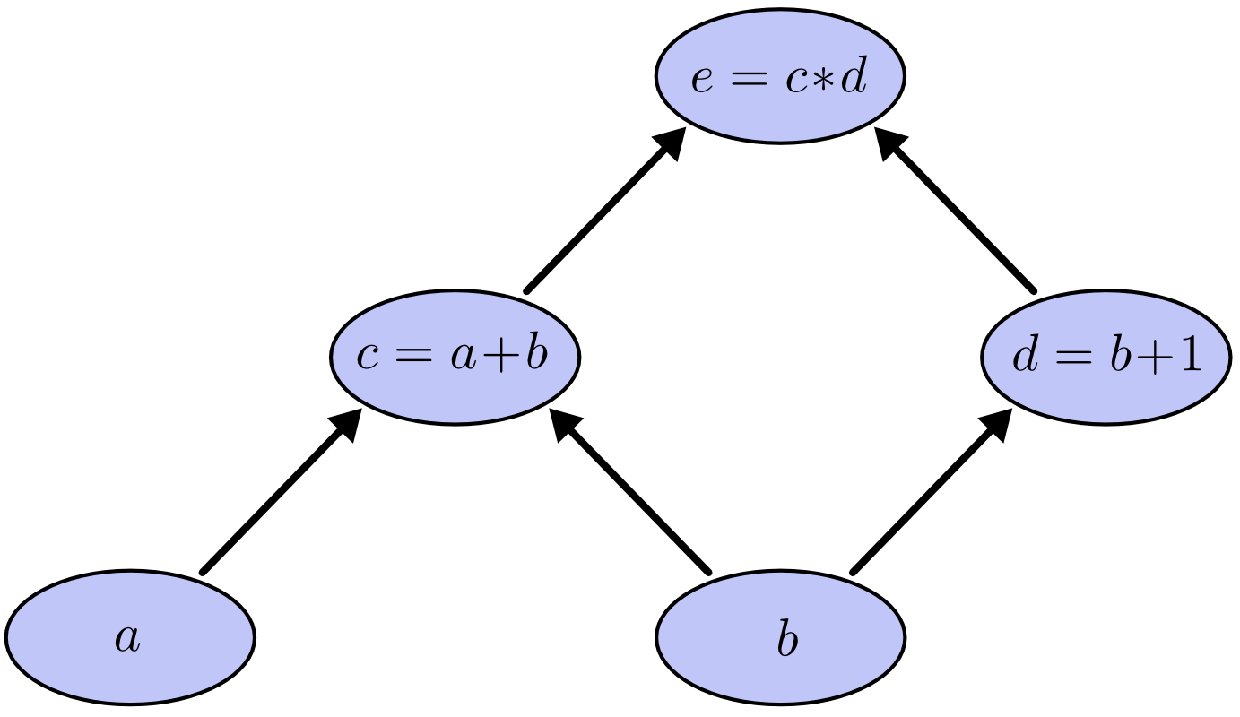
Fig 1.a: A basic computational graph, courtesy Christopher Olah
- We can evaluate the expression by setting the input variables (i.e. nodes with only outputs) to certain values and computing nodes up through the graph.
In the example below, if we plug \(a = 2\) and \(b = 1\), we get the output \(e = 6\).
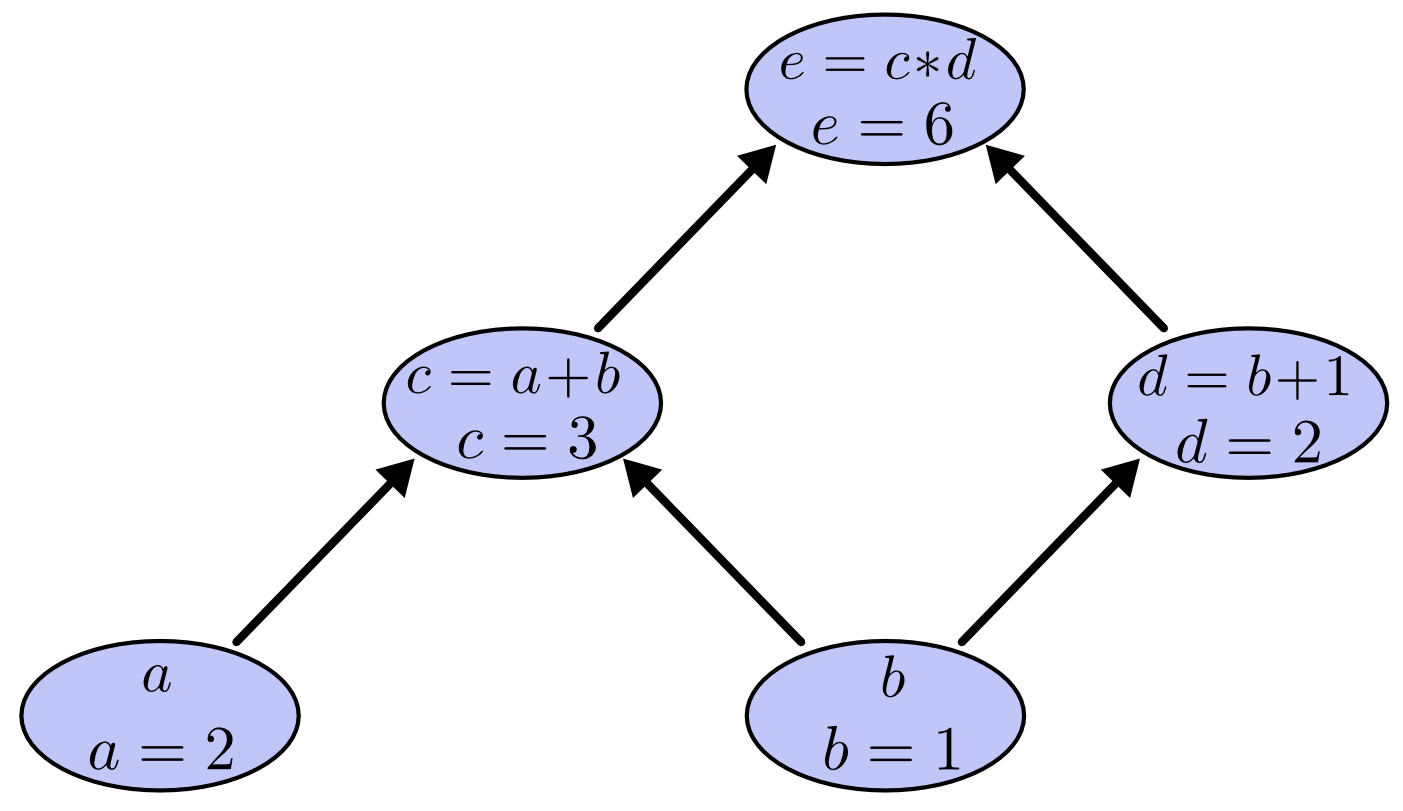
Fig 1.b: Calculating the output of a computational graph, courtesy Christopher Olah
Derivatives on Computational Graphs
Derivatives (also called gradients) on computational graphs are a bit more tricky to understand. I will deviate from Colah’s explanation and provide multiple, more explicit examples geared towards neural networks.
You are encouraged to work through the following examples, without looking at the answer right away. Each takes about 5 minutes using a pen and paper.
Example: a comprehensive Computational Graph
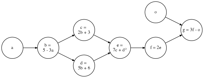
Fig 2.a: Example computational graph
Consider the graph above. Here, the output is \(g = 3f - o\), and each of the nodes calculates a function of their input, which is then passed on to the next node(s).
Now, suppose we want to calculate the partial derivative i.e. gradient of the output \(g\), with respect to each variable, i.e. we want to know: \(\frac{\partial g}{\partial g}\), \(\frac{\partial g}{\partial o}\), \(\frac{\partial g}{\partial f}\), \(\frac{\partial g}{\partial e}\), \(\frac{\partial g}{\partial d}\), \(\frac{\partial g}{\partial c}\), \(\frac{\partial g}{\partial b}\), \(\frac{\partial g}{\partial a}\)
The first few are easy:
\[\begin{split}\frac{\partial g}{\partial g} &= 1 & \\ \frac{\partial g}{\partial f} &= \frac{\partial (3f - o)}{\partial f} &= 3 \\ \frac{\partial g}{\partial o} &= \frac{\partial (3f - o)}{\partial o} &= -1\end{split}\]
However, as we move further towards the inputs of the graph, it gets more complicated:
Let’s try to compute \(\frac{\partial g}{\partial e}\). We have:
\[\begin{split}\frac{\partial g}{\partial e} &= \frac{\partial (3f-o)}{\partial e} \\ &= \frac{\partial (3(2e)-o)}{\partial e} \\ &= \frac{\partial (6e-o)}{\partial e} \\ &= 6\end{split}\]It starts to get repetitive when computing \(\frac{\partial g}{\partial d}\):
\[\begin{split}\frac{\partial g}{\partial d} &= \frac{\partial (3f-o)}{\partial d} & \text{(repeated calculation)} \\ &= \frac{\partial (3(2e)-o)}{\partial d} & \text{(repeated calculation)} \\ &= \frac{\partial (6e-o)}{\partial d} & \text{(repeated calculation)} \\ &= \frac{\partial (6(7c + d^2) -o)}{\partial d} \\ &= \frac{\partial (42c + 6d^2 -o)}{\partial d} \\ &= \frac{\partial (42c)}{\partial d} + \frac{\partial (6d^2)}{\partial d} - \frac{\partial (o)}{\partial d} \\ &= 12d\end{split}\]- Notice in the example above, when we are computing \(\frac{\partial g}{\partial d}\) from scratch, the first few steps are essentially repeated from our calculation of \(\frac{\partial g}{\partial e}\).
To save effort, we can use the chain-rule of partial derivatives to re-use the value of \(\frac{\partial g}{\partial e}\) which we had obtained, to calculate \(\frac{\partial g}{\partial d}\).
By chain rule, we have \(\frac{\partial g}{\partial d} = \frac{\partial g}{\partial e}\cdot \frac{\partial e}{\partial d}\)
We had already calculated \(\frac{\partial g}{\partial e} = 6\).
With a tiny bit of extra calculation:
\[\begin{split}\frac{\partial g}{\partial d} &= 6 \left( \frac{\partial (7c + d^2)}{\partial d} \right) \\ &= 12d & \text{(what we want)} \\ &= 12(5b + 6) = 60b + 72 \\ &= 60(5 - 3a) + 72 \\ &= 372 - 180a\end{split}\]Thus, \(\frac{\partial g}{\partial d} = 12d\), the same answer we got before.
- If the above process seems familiar to dynamic programming, it’s because that’s exactly what it is!
We store the partial derivatives (also called “gradients”) which we had computed earlier, and use those to calculate further gradient values.
Note that we can only do so while moving from the outputs towards the inputs of the graph, i.e. “backwards” from the normal flow of data.
- Note that for \(\frac{\partial g}{\partial d}\), unlike the previous gradients, we obtain the answer in terms of the input \(a\).
- If you have taken a calculus class, you might have been asked to calculate the “partial derivative of \(y\) with respect to \(x\), at point \((t=0.5)\)”, represented by \(\frac{\partial y}{\partial x}|_{(t=0.5)}\), where \(y\) is a function of \(x\), which is itself a function of \(t\) i.e. \(y=f_1(x)\) and \(x=f_2(t)\).
This value is calculated by computing \(\frac{\partial y}{\partial x}\), obtaining it as a function of \(t\), and then substituting \((t=0.5)\) to obtain a scalar value.
Similarly, we can plug the values of \(a\) into the equation \(\frac{\partial g}{\partial d}\) above:
\[\begin{split}\frac{\partial g}{\partial d}|_{(a=0.5)} &= 62 - 30(0.5) \\ &= 62 - 15 \\ &= 47\end{split}\]
- Also note that, we can choose how far we want to “unroll” the final value.
We could have stopped at \(12d\) OR \(60b + 72\), and used it to calculate \(\frac{\partial g}{\partial d}|_{(d=\dots)}\) OR \(\frac{\partial g}{\partial d}|_{(b=\dots)}\), respectively. Which one we would chooose depends on whether we had the values of \(d\) or \(b\) pre-computed.
- We can now confidently use chain-rule to calculate \(\frac{\partial g}{\partial c}\).
Since \(c\) is only consumed by \(e\) (i.e. \(c\)’s only dependent is \(e\)), we have:
\[\begin{split}\frac{\partial g}{\partial c} &= \frac{\partial g}{\partial e} \cdot \frac{\partial e}{\partial c} \\ &= 6 \cdot \frac{\partial (7c + d^2)}{\partial c} = 6(7) \\ &= 42\end{split}\]
- Let’s continue with our example, and calculate the value of \(\frac{\partial g}{\partial b}\). But if we look at the diagram, \(b\) feeds into both \(c\) and \(d\)…which one do we pick as the “precomputed” value?
The answer is: both. In this situation, we must use an extension of the normal chain rule, called Multivariable Chain rule (with a single input variable).
Under Multivariable chain rule, to get the partial derivative of \(g\) with respect to \(b\), we must take the sum of products of gradients along all possible paths, traced backwards from \(g\) to \(b\).
From the graph, there are two paths from \(g\) to \(b\): \(g \rightarrow f \rightarrow e \rightarrow d \rightarrow b\) and \(g \rightarrow f \rightarrow e \rightarrow c \rightarrow b\).
Thus, we have:
\[\begin{split}\frac{\partial g}{\partial b} &= \left( \frac{\partial g}{\partial f} \cdot \frac{\partial f}{\partial e} \cdot \frac{\partial e}{\partial d} \cdot \frac{\partial d}{\partial b} \right) + \left( \frac{\partial g}{\partial f} \cdot \frac{\partial f}{\partial e} \cdot \frac{\partial e}{\partial c} \cdot \frac{\partial c}{\partial b} \right) \\ &= \left( \frac{\partial g}{\partial d} \cdot \frac{\partial d}{\partial b} \right) + \left( \frac{\partial g}{\partial c} \cdot \frac{\partial c}{\partial b} \right)\end{split}\]Let us first calculate \(\frac{\partial d}{\partial b}\) and \(\frac{\partial c}{\partial b}\) separately (you’ll see why in a second):
\[\begin{split}\frac{\partial d}{\partial b} &= \frac{\partial (5b + 6)}{\partial b} &= 5 \\ \frac{\partial c}{\partial b} &= \frac{\partial (2b + 3)}{\partial b} &= 2\end{split}\]We can now simply plug in all the values:
\[\begin{split}\frac{\partial g}{\partial b} &= \left( \frac{\partial g}{\partial d} \cdot \frac{\partial d}{\partial b} \right) + \left( \frac{\partial g}{\partial c} \cdot \frac{\partial c}{\partial b} \right) \\ &= (12d \cdot 5) + (42 \cdot 2) \\ & = 60d + 84 & \text{(what we want)} \\ &= 60(5b + 6) + 84 \\ &= 300b + 444 \\ &= 300(5 - 3a) + 444 \\ &= 1944 - 900a\end{split}\]We can also verify that the Multivariable chain rule is correct by computing from scratch:
\[\begin{split}\frac{\partial g}{\partial b} &= \frac{\partial (3f-o)}{\partial b} \\ &= \frac{\partial (6e - o)}{\partial b} \\ &= \frac{\partial (42c + 6d^2 - o)}{\partial b} \\ &= 42 \left( \frac{\partial c}{\partial b} \right) + 12d \left( \frac{\partial d}{\partial b} \right) - \frac{\partial (o)}{\partial b} \\ &= 42(2) + 12d(5) - 0 \\ &= 60d + 84\end{split}\]…which is what we had obtained using the Multivariable chain rule.
Gradient-flow graph for example computational graph
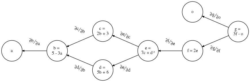
Fig 2.b: Gradient-flow graph for above example
- We can think of the above computation as gradients (i.e. partial derivatives) flowing from the output(s) towards the input(s) of a computational graph, and construct the respective gradient-flow graph, shown in Fig 2.b: Gradient-flow graph for above example.
In this graph, the edges represent the partial derivative between the two nodes connected by the edge.
To get the gradient of a particular node w.r.t. the output, we consider gradients along all paths from the output to that node.
- As we traverse edges along a particular path from the output to the input, we multiply by the gradients we encounter.
E.g. to get \(\frac{\partial g}{\partial e}\), we multiply \(\frac{\partial g}{\partial f} \cdot \frac{\partial f}{\partial e}\)
As for \(\frac{\partial g}{\partial c}\): despite the fork at \(e\), there is only one path from \(g\) to \(c\), which is \(g \rightarrow f \rightarrow e \rightarrow c\) . Thus:
\[\frac{\partial g}{\partial c} = \frac{\partial g}{\partial f} \cdot \frac{\partial f}{\partial e} \cdot \frac{\partial e}{\partial c}\]The same holds true for \(\frac{\partial g}{\partial d}\).
When two or more paths in a gradient-flow graph join at a node (such as \(b\)) we must sum up the product of gradients along all of these paths:
\[\frac{\partial g}{\partial b} = \left( \frac{\partial g}{\partial f} \cdot \frac{\partial f}{\partial e} \cdot \frac{\partial e}{\partial d} \cdot \frac{\partial d}{\partial b} \right) + \left( \frac{\partial g}{\partial f} \cdot \frac{\partial f}{\partial e} \cdot \frac{\partial e}{\partial c} \cdot \frac{\partial c}{\partial b} \right)\]A more intuitive grouping is possible, based on the flow:
\[\frac{\partial g}{\partial b} = \frac{\partial g}{\partial f} \cdot \frac{\partial f}{\partial e} \cdot \left( \frac{\partial e}{\partial d} \cdot \frac{\partial d}{\partial b} + \frac{\partial e}{\partial c} \cdot \frac{\partial c}{\partial b} \right)\]The term in the parenthesis above represents the subgraph \(bcde\), which forks at \(e\) and joins at \(b\). We can calculate the gradient of such subgraphs as an independent block:
\[\frac{\partial e}{\partial b} = \frac{\partial e}{\partial d} \cdot \frac{\partial d}{\partial b} + \frac{\partial e}{\partial c} \cdot \frac{\partial c}{\partial b}\]
We can actually use the gradient-flow graph to get the partial derivative of any variable (not just the final output) with respect to any variable it depends on.
E.g. if we wanted \(\frac{\partial f}{\partial d}\), we would just have to look at the edges along all paths from \(f\) to \(d\) and trace the path of gradients accordingly:
\[\frac{\partial f}{\partial d} = \frac{\partial f}{\partial e} \cdot \frac{\partial e}{\partial d}\]- Let us now use our knowledge to calculate \(\frac{\partial g}{\partial a}\).
Peeking at the gradient flow graph, we see that there is only one gradient flowing into \(a\). This, we can use our basic chain rule:
\[\begin{split}\frac{\partial g}{\partial a} &= \frac{\partial g}{\partial b} \cdot \frac{\partial b}{\partial a} \\ &= (1944 - 900a)(-3) \\ &= 2700a - 5832\end{split}\]Remember: we store and re-use the values we had already calculated. To obtain any new gradient value, we only have to calculate the gradient on each of the final edge incoming to the target node, on the gradient-flow graph. Here, that is \(\frac{\partial b}{\partial a}\). We then reuse the already-computed values of gradients to fill the rest of the chain (here, \(\frac{\partial g}{\partial b}\)).