Feedforward step of a basic feedforward neural network
What is feedforward?
The feedforward step for a neural network is when we pick a sample \(D_i\) from the dataset \(D\), and feed it into the network.
The network’s weights in each layer tranform the sample from its initial representation into various other representations, which are fed into layer after layer.
The output of the final hidden layer, \(Z_{L-1}\), is then transformed by the output layer to create the network output \(O\).
Differences in feedforward during training
During training, two additional steps are
While the input propagates through a layer, we also calculate and store the gradients of the output with respect to the weights of that layer.
While training, can also calculate the value of the error function, \(E(o, Y_i)\).
Vectorized feedforward with a single sample
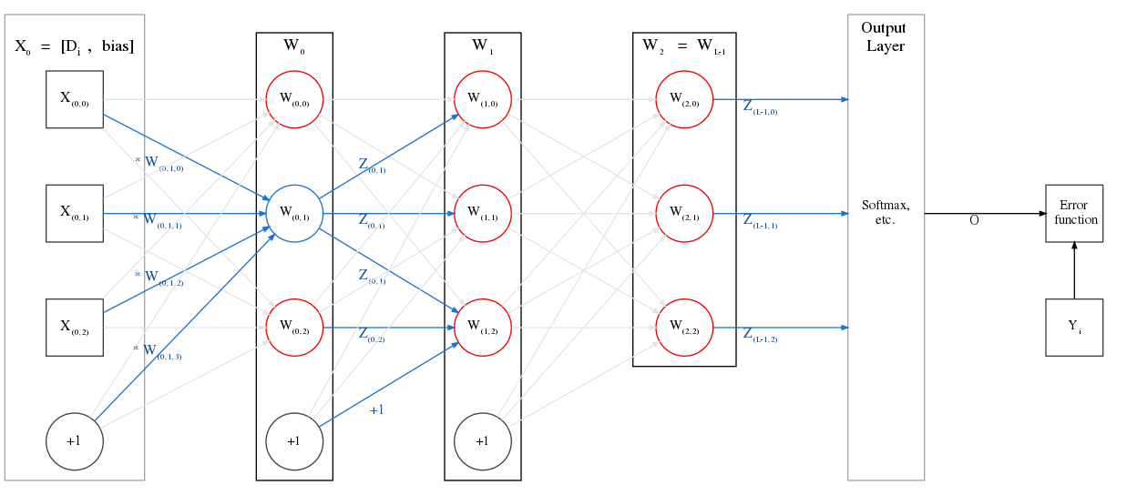
Basic Feedforward Neural Network
Consider the example network above.
Suppose we have a dataset \(D = D_0 \dots D_{N-1}\), and each sample is represented by 3 features.
Assume we randomly pick the \(38^{th}\) sample in the dataset to feed to our network: \(D_{37} = \left[\begin{array}{ccc} 3 & -5 & 12 \end{array}\right]\)
The input (row) vector to the network is \(X_0\), which will have 4 features. The final one will be the bias value, +1, which we concatenate to \(D_{37}\). \(X_0 = \left[\begin{array}{cc} D_{37}, & +1 \end{array}\right] = \left[\begin{array}{cccc} 3 & -5 & 12 & +1 \end{array}\right]\)
- Each layer in a basic feedforward network can be represented by a matrix.
In the example above, \(W_0\) has 3 neurons, each of which takes 4 inputs, and thus we can represent it as a \(4 \times 3\) matrix, where each column is a neuron. The final row of each layer is the weights corresponding to the bias of the input \(X_0\). E.g.
\[\begin{split}W_0 = \left[\begin{array}{cccc} 0.3073 & -3.31913 & -2.455 \\ -0.121 & -2.149 & 0.041 \\ -4.2342 & 5.6798 & 0.6527 \\ -3.6295 & 12.88588 & -0.499 \end{array}\right]\end{split}\]
We compute the vector-matrix multiplication of these two to get the affine of the first layer, i.e.
\[\begin{split}A_0 &= X_0 \cdot W_0 \\ &= \left[\begin{array}{ccc} -52.913 & 81.83109 & -0.2366 \end{array}\right]\end{split}\]To compute the output of the first layer, we apply the activation function to each element of the affine vector:
\[\begin{split}Z_0 &= sig(A_0) \\ &= \left[\begin{array}{ccc} sig(-52.913) & sig(81.83109) & sig(-0.2366) \end{array}\right] \\ &\approx \left[\begin{array}{ccc} 0 & 1 & 0.441 \end{array}\right]\end{split}\]Here, we have chosen the sigmoid activation function, i.e.
\[sigmoid(x) = sig(x) = \frac{1}{1+e^{-x}}\]
We’re not done yet! \(Z_0\) is the output from the layer \(W_0\), but to get \(X_1\), the input to layer \(W_1\), we must concatenate a bias value of +1 to the end of \(Z_0\).
\[\begin{split}X_1 &= \left[\begin{array}{cc} Z_0, & +1 \end{array}\right] \\ &= \left[\begin{array}{cccc} 0 & 1 & 0.441 & +1 \end{array}\right]\end{split}\]We pass this as the input to layer \(W_1\), which is also a \(4 \times 3\) matrix, and similarly obtain \(Z_1\) and \(X_2\).
\[\begin{split}X_2 &= \left[\begin{array}{cc} Z_1, & +1 \end{array}\right] \\ &= \left[\begin{array}{cc} activation(X_1 \cdot W_1), & +1 \end{array}\right]\end{split}\]Similarly, we compute all the way until we get \(Z_{L-1}\). In the example above, that is \(Z_2\).
\[Z_2 = \left[ \begin{array}{cc} activation(\left[\begin{array}{cc} activation(\left[\begin{array}{cc} activation(X_0 \cdot W_0), & +1 \end{array}\right] \cdot W_1), & +1 \end{array}\right] \cdot W_2) \end{array} \right]\]- We feed the output of the final layer into the output layer, where an output function computes the output of the network, \(O\).
\(Z_{L-1}\) does not have a bias unit concatenated to it when we feed it to the output layer.
- For the example above, assume we are performing multi-class classification, with \(K=3\) output classes.
Let \(Z_{L-1} = Z_2 = \left[\begin{array}{ccc} 0.2 & 0.0013 & 0.998 \end{array}\right]\)
- We will use the Softmax function to convert our outputs into a probability distribution over the 3 classes.
For the \(i^{th}\) element in \(Z_{L-1}\), we obtain the Softmax value as:
\[Softmax(Z_{L-1}, i) = \frac{ e^{Z_{(L-1, i)}} }{ \sum_{k=0}^{K-1} \left( e^{Z_{(L-1, {} k)}} \right) }\]i.e. we normalize the exponentials of \(Z_{L-1}\).
We calculate each of these and put them into a vector:
\[Softmax(Z_{L-1}) = \left[\begin{array}{c} Softmax(Z_{L-1}, i) \end{array}\right]_{i=0}^{K-1}\]The softmax vector sums to \(1\), so each value can be considered the probability of belonging to the corresponding class, as predicted by our network.
Applying the softmax operation to \(Z_2\), we obtain the network output, \(O\):
\[O = Softmax(Z_2) = \left[\begin{array}{ccc} 0.2474 & 0.2029 & 0.5497 \end{array}\right]\]
- We need to calculate how (in)accurate our network’s output was. For this, we use an Error function, \(E\).
In our problem, there are \(K=3\) classes: \(0, 1, 2\).
Let’s assume the correct class for \(D_{37}\) was the third one, i.e. \(Y_{37} = 2\). * We can’t directly compare our output vector with this value. So instead, we use a mechanism known as one-hot encoding and convert \(Y_{37}\) into the vector \(\left[\begin{array}{ccc} 0 & 0 & 1 \end{array}\right]\). The third element is \(1\), meaning our example \(D_{37}\) belongs to the third class.
- Let’s use the Squared Error function to calculate how different our network’s prediction \(O\) is from the actual output from the dataset i.e. \(Y_{37}\).
Squared Error:
\[E(O, Y_i) = \frac{1}{2} \cdot \sum_{k=0}^{K-1} {\left( O_k - Y_{(i, k)} \right)}^2\]i.e. we sqaure the differences between each element of the predicted output, and the actual output. This value is always positive.
In the example above, we get squared error value as:
\[\begin{split}E &= \frac{1}{2} \cdot \left( (0.2474 - 0)^2 + (0.2029 - 0)^2 + (0.5497 - 1)^2 \right) \\ &= 0.1526\end{split}\]