Notation and terminology for feedforward neural networks
When you deal with neural networks, it is easy to lose track of which exact neuron or layer is being referred to in the discussion. For this reason, I use the notation described in the sections below, which is hopefully unambiguous.
Indexing
I will use zero-indexing everywhere, as it makes things easier to translate into code.
Dataset and batches
While training the network weights, we provide a dataset \(D\).
The network’s job is to fit the dataset well and reduce the error on training samples.
The dataset has \(N\) samples.
- Each sample in this dataset is an input-output pair, denoted (\(D^{(i)}\), \(Y^{(i)}\)) or (\(d^{(i)}\), \(y^{(i)}\))
- \(D^{(i)}\) (the input part of the \(i^{th}\) sample) is a vector/tensor.
The parenthesis in the superscript is to help us differentiate this from the “\(i^{th}\) power” notation. If we want to index certain components of the input, we will use the subscript notation.
E.g. if our dataset consists of black-and-white images, each of which is 32x32 pixels across, and where each pixel takes is a grey value between 0 and 127, then we can represent each sample’s input as a 32x32 matrix of variables, i.e. \(D^{(i)} \in \mathbb{R}^{(32, 32)}\). If we want the grey value at the \(3^{th}\) row and \(5^{th}\) column of the \(9^{th}\) image, we would index it as: \(D^{(8)}_{(2, 4)}\) (remember, we use zero-indexing).
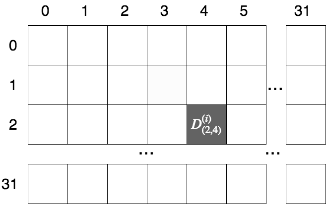
Indexing a 32x32 image matrix
- \(Y^{(i)}\) is the output part of the \(i^{th}\) sample. It is also known as the target or the ground truth value.
For regression problems, \(Y_{(i)}\) will be a scalar. E.g. if we are performing housing-price prediction, \(Y^{(10)} = 598\) might mean that the price of the \(11^{th}\) house is $598,000.
For classification problems, \(Y^{(i)}\) will belong to one (or more) of \(K\) classes or
labels. E.g. for single-label image classification, \(Y^{(7)} = Cat\) means that the \(8^{th}\) image is actually a cat. Whereas if our problem is multi-label classification, we might have \(Y^{(31)} = \begin{matrix} \{Cat, & Dog, & Horse\} \end{matrix}\), meaning our sample actually contains a cat, dog and a horse.
During classification, an important representation of each target variable is one-hot encoding. In this representation, we assign each of the \(K\) possible classes to index of a vector, and every target thus becomes a vector of ones and zeros, depending on whether that class is present in the sample or not.
- E.g. Suppose we have a multi-label image classification problem, where we have the classes \(\begin{matrix} \{Bear, & Cat, & Dog, & Goose, & Horse, & Mouse, & Zebra\} \end{matrix}\) \((K = 7)\). For each class which is present, we set the value of 1 in its respective index in this array. Following this procedure, the above two targets become:
- \[\begin{split}Y^{(7)} = Cat = \left[ \begin{matrix} 0 \\ 1 \\ 0 \\ 0 \\ 0 \\ 0 \\ 0 \end{matrix} \right] \\ Y^{(31)} = \begin{matrix} \{Cat, & Dog, & Horse\} \end{matrix} = \left[ \begin{matrix} 0 \\ 1 \\ 1 \\ 0 \\ 1 \\ 0 \\ 0 \end{matrix} \right]\end{split}\]
- If we are going to split the dataset into batches for training (as in the case of batched gradient descent), we will let \(B\) will denote the batch size.
Generally \(B \lt\lt N\), e.g. we have a dataset of 1 million samples, but we train in batches of 128 at a time.
Every time we train over the entire dataset (i.e. we train using \(\frac{N}{B}\) batches), it is called an epoch.
Note: the network performs the same computation on each sample in the batch. Thus, most network-level operations (prediction, feedforward, backpropagation, etc) can be run in parallel over the samples in a batch.
Network terminology
Neurons
The most vanilla form of a neural network is a sequence of layers, each of which is a stack of neurons. A neuron is the basic unit of computation in a neural network.
We say that neuron “owns” a vector of weights. It takes as input a vector from the previous layer, along with a linear bias, and computes the dot product of these two vectors (this operation is called an affine transform). This scalar affine value is then transformed by a non-linear activation function (denoted \(f(x)\)) to obtain another scalar value, which is the neuron’s output.
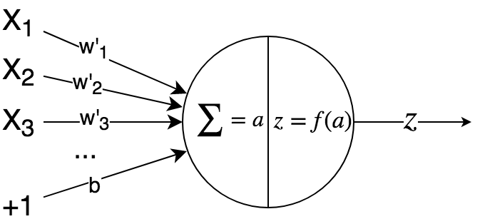
Basic Neuron
- Let’s do this mathematically. The affine value is:
- \[a = w' \cdot X + b = \left(\sum_{i=0}^{n-1}(w'_i \cdot X_i) \right) + b\]
- and the neuron output is:
- \[z = f(a)\]
Where:
\(X\) = input vector to neuron (this comes from the previous layer).
\(w'\) = weight vector of neuron.
\(b\) = bias unit value (this value is learnt during training).
\(f\) = the activation function. E.g. sigmoid, tanh, ReLU, etc.
During training, we learn the values of the vector \(w'\) and the scalar \(b\) together, so we usually concatenate them into a single vector: \(w = [\begin{matrix} w',& b \end{matrix}]\). Going forward, I will use \(w\) to mean this concatenated vector.
Layer inputs
Remember: we draw samples from the dataset \(D\) and feed them into network for training/prediction. Each sample is an input-target pair \((D^{(i)}, Y^{(i)})\).
- We might also feed the network batches of \(B > 1\) samples at a time:
- \[\begin{split}\left[ \begin{matrix} D^{(i)}, & Y^{(i)} \\ D^{(i+1)}, & Y^{(i+1)} \\ \dots & \dots \\ D^{(i+B-1)}, & Y^{(i+B-1)} \end{matrix} \right]\end{split}\]
Regardless of whether we feed a single sample or a batch, we will use \(X_l\) or \(x_l\) to denote the inputs to a layer \(H_l\). We will rely on the context to tell us the dimensionality of \(X_l\).
Thus, the input to the first layer will be \(X_0 = \begin{matrix} D^{(i)}, & +1 \end{matrix}\).
For subsequent layers, the layer inputs are \(X_1, X_2, \dots, X_{L-1}\).
Layer outputs
As mentioned, each neuron uses the layer input and its own weights to calculate the affine value, which it then passes through a non-linear activation function to create the neuron output.
We will denote the output from the \(j^{th}\) neuron of the \(l^{th}\) layer as \(Z_{(l, j)}\) or \(z_{(l, j)}\).
When required, we will denote the value of just the affine computation of the corresponding neuron as \(A_{(l, j)}\) or \(a_{(l, j)}\). Other sources might refer to this as \(net_{(l, j)}\).
Grouping the outputs of all neurons in a layer, we get the layer output, which is a vector \(Z_l \in \mathbb{R}^{|H_{l}|}\).
Note:
For simple, dense networks, the output of each hidden layer (along with a bias value) becomes the input to the next later.
i.e. \(X_{l+1} = [\begin{matrix} Z_{l}, & +1 \end{matrix}]\). The comma here means we concatenate the vector \(Z_l\) with the scalar bias value (which is usually +1) to create a new vector, which we feed into the subsequent layer.
In the case of recurrent networks, the input of each layer is not only the output of the previous layer in the network, but also the output of the same layer in the previous time step (i.e. for the previous sample \(D^{(i-1)}\)).
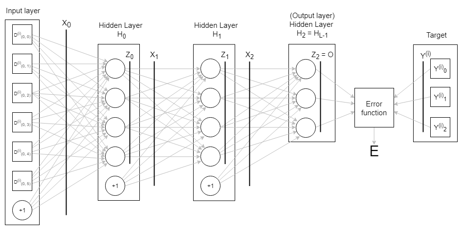
Basic Neural Network
Final (“output”) layer and network output
The final hidden layer of a network is frequently referred to as the “output” layer of the network.
This is very different from the network output! The output layer produces the network output, i.e. when we use the network to train/predict, the output layer tells us what the network predicts for a particular sample’s input, \(D^{(i)}\).
We will denote the output layer as \(H_{L-1}\) and the network output as \(O\). As the output layer is the final hidden layer, we have \(O = Z_{L-1}\).
Some important points:
The network output \(O\) does not have the bias value +1 concatenated to it. This is because the output layer is the final layer, and there are no trainable weights “after” it.
- In general, when we design basic (dense) networks, we maintain the same number of neurons in each hidden layer. The output layer is the exception to this rule: the network output \(O\) must have the same dimensions as the sample’s target, \(Y^{(i)}\). This is because both of these will be fed into the Error function, which computes how much they differ from each other.
If we have a regression problem, \(O, Y^{(i)} \in \mathbb{R}\) i.e. both are scalars.
If we have a classification problem and we using one-hot encoding to obtain a vector \(Y^{(i)}\), then \(O, Y^{(i)} \in \mathbb{R}^K\), where \(K\) is the number of classes.
Error function
The Error function, also called the Loss function or Cost function, tells us how much the network’s prediction differs from the sample’s actual target. That is, it tells us how much \(O\) and \(Y^{(i)}\) differ.
We denote the Error function by \(E(O, Y^{(i)})\), or just \(E\) for short.
The Error function always outputs a scalar i.e. \(E \in \mathbb{R}\). The neural network training algorithm (gradient descent etc.) attempts to iteratively tweak the weights, so as to minimize the error value predicted for the training dataset.
Some common error functions are Mean-squared error and Categorical cross-entropy.
Example usage of notation and terminology
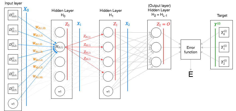
Basic Neural Network example
Let’s go apply what we have just learned to the figure above.
We see that:
\(L = 3\) i.e. there are three (hidden) layers.
\(Y^{(i)} \in \mathbb{R}^3\), i.e. we have \(K=3\) output classes.
The input to the network, \(D^{(i)}\), is a vector with 6 features, i.e. \(D^{(i)} \in \mathbb{R}^{6}\). When combined with a bias value +1, this becomes \(X_0 \in \mathbb{R}^{7}\). This is the input vector that is fed into each neuron of the first hidden layer \(H_0\).
\[X_0 = \left[ \begin{matrix} D_{(0,0)} & D_{(0,1)} & D_{(0,2)} & D_{(0,3)} & D_{(0,4)} & D_{(0,5)} & +1 \end{matrix} \right]\]Each neuron in the network owns a vector of weights, which it uses to produce the output. In the figure above, we consider \(H_{(0, 1)}\), i.e. the second neuron of \(H_0\). This neuron owns the following weight vector:
\[\begin{split}W_{(0, 1)} = \left[ \begin{matrix} W_{(0, 1, 0)} \\ W_{(0, 1, 1)} \\ W_{(0, 1, 2)} \\ W_{(0, 1, 3)} \\ W_{(0, 1, 4)} \\ W_{(0, 1, 5)} \\ W_{(0, 1, 6)} \end{matrix} \right]\end{split}\]Taking the dot product of the input vector and the weight vector (not shown in the figure), we obtain the affine value \(A_{(0,1)} = X_0 \cdot W_{(0,1)}\).
Passing this through the activation function, we get the corresponding neuron output, \(Z_{(0,1)} = f(A_{(0,1)})\). This is sent to all neurons in the subsequent layer.
Note that \(A_{(0,1)} \in \mathbb{R}\) and \(Z_{(0,1)} \in \mathbb{R}\), i.e. both are scalars.
\(Z_0\), the vector of outputs of all neurons in the first layer \(H_0\), is combined with a bias value +1 and becomes the next layer’s input. From the example above: \(X_{1} = [ \begin{matrix} Z_{0}, & +1 ] \end{matrix} = [ \begin{matrix} Z_{(0,0)} & Z_{(0,1)} & Z_{(0,2)} & Z_{(0,3)} & +1 \end{matrix} ]\).
We follow a similar process for layers \(H_1\) and \(H_2\).
The output layer \(H_2\) calculates the network output \(Z_{2} = O\), which is consumed by the error function, along with the one-hot encoded target vector, \(Y^{(i)}\). This produces the error value \(E\) for the sample \((D^{(i)}, Y^{(i)})\).